Lab Members: Carol Ge, Katie Diventi, & Muskan Manchanda
Research Question: How does time affect the position of a cart on a ramp?
Variables & Controls of the ExperimentVariables
Controls
|
MethodsTo Control the Variables:
Start off by selecting a smooth, flat ramp that is slightly elevated on one end for the cart to travel down. This way, its movement will not be influenced by factors other than the angle of the ramp it is on. Let the cart go without pushing it at the end of the elevated end of the ramp so it rolls down to the other side of the ramp. To Collect the Data:
Set up a phone on a stable surface so that its camera captures the entire ramp, including the starting position and final position, as well as a meter stick at the same angle and next to the ramp. Afterwards, insert the video into the Logger Pro application to manually calibrate the initial time at 0, the release point as the origin, and the angle of the axes to set up the proper preparations for capturing data points. To measure the distance travelled by the cart, calibrate the scale along the known length of an object, which in this case is the meter stick. By adding a dot for the position of the cart at each frame on Logger Pro, one can carefully plot out the position of the cart at specific time points on a position-time graph. |
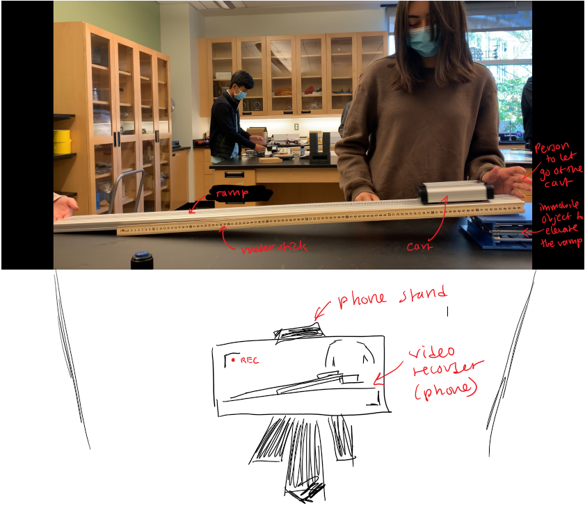
Labeled Diagram of the Cart on the Ramp Video lab Set-Up
Procedure
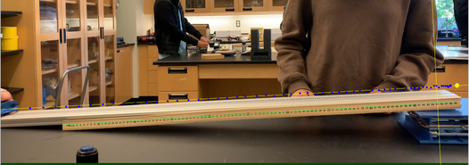
After placing the cart at the initial position on the elevated edge of the ramp, we captured a video with an iPhone camera of the cart rolling down to the edge on the table. Muskan let go of the cart and Katie caught it while I was monitoring the video recording. This video was subsequently analyzed with Logger Pro to identify the position in meters of the cart from 0 to 2 seconds, which was then used to identify the velocity. We only did one trial of the cart rolling down the ramp because only one video was necessary to capture its motion.
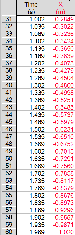
Raw Data - Table*The data tables below are part of the same data table -- first part (left) and second part (right)*
|
Raw Data - Graphical Representation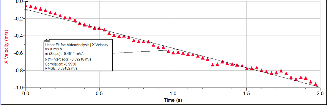
The image pictured above is a position-time graph, which was generated by the Logger Pro application. The slope of this graph indicates that the horizontal position of the cart was decreasing. The y-intercept of the graph indicates the position the cart is at when the time is 0, which is 0.051 meters. The quadratic model was the best fit for this graph as the slope was getting steeper, indicating that the cart was speeding up as time increased.
|
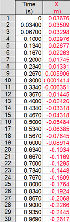
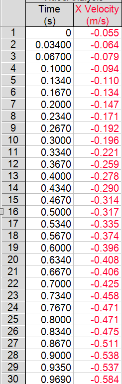
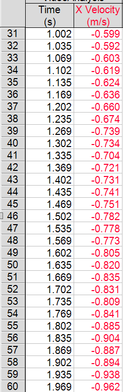
Processed Raw Data - Table*The data tables below are part of the same data table -- first part (left) and second part (right)*
|
Processed Raw Data - Graphical Representation
The image pictured above is a velocity-time graph, which was generated by the Logger Pro application with the position and time data. The slope of this graph indicates that the cart was speeding up at a rate of approximately -0.4511 m/s/s as the absolute value of the velocity is increasing. The y-intercept of the graph indicates the initial velocity of the cart, which is -0.092 meters per second. The linear model was the best fit for this graph as the slope of the velocity-time graph was getting steeper, indicating that the cart was accelerating.
Equation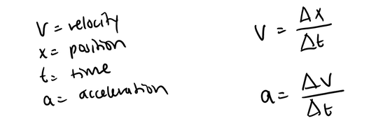
|
Conclusion
In this lab, we identified that the velocity of an object traveling on a smooth ramp with an initial velocity of 0 m/s speeds up, or accelerates, as time goes on.
This lab’s purpose was to identify the correlation between change in velocity and change in time, which we determined to be acceleration. Unlike the buggy lab, the velocity was changing and did not remain roughly constant. By looking at the position-velocity graph, we noticed that the change in the horizontal position roughly aligned with a quadratic model with a negative slope. Moreover, the slope was becoming steeper, indicating that the cart was accelerating, which was able to be represented by a velocity-time graph that roughly aligned with a linear model. It should be noted that the cart was traveling towards the left, so the horizontal position was negative.
In addition, the Logger Pro tools we used to measure position from a video show us how modern technological tools can produce more accurate measurements than humans because there is no need to account for a reaction time that delays measurements and decreases the accuracy. We can also gather more data points from a single trial by using a video.
With our knowledge from this lab, we can now assess the velocity and acceleration of any moving object that is speeding up, whether in a straight line on a flat plane or on an incline. We can use this knowledge to measure the velocity and acceleration of the movement in a vast amount of scenarios in real life, such as a car speeding up from 0 mph to 25 mph after a red light, or some people sledding down a hill and speeding up as time goes on.
Evaluating Procedures
Weaknesses and Limitations
The main weakness/ limitation is that we are limited by the technology that we have. We are only able to generate as much data as we can gather given the available resources, specifically how many frames the video camera can capture.
Uncertainty
Improvement
To improve this lab, I would gather data over a longer period of time by using a longer ramp with the same angle of incline. A camera that could capture more frames per second would also help to increase the amount of data. This way, we could have more data to work with when generating position-time graphs and velocity-time graphs. With these graphs, we can see if our quadratic and linear models, respectively, still roughly align with the data to make further predictions.
The main weakness/ limitation is that we are limited by the technology that we have. We are only able to generate as much data as we can gather given the available resources, specifically how many frames the video camera can capture.
Uncertainty
- The plotting of each point for the horizontal position of the cart was not entirely accurate because for some specific frames, the picture would be a little blurry so it was a little difficult to locate the precise position of the cart. We can tell by the y-intercept of the velocity-time graph not being 0 m/s.
- The initial time that the cart began rolling down the ramp was difficult to determine due to its slow motion, as well as the experimenter’s hand slightly covering the cart as they let it go.
Improvement
To improve this lab, I would gather data over a longer period of time by using a longer ramp with the same angle of incline. A camera that could capture more frames per second would also help to increase the amount of data. This way, we could have more data to work with when generating position-time graphs and velocity-time graphs. With these graphs, we can see if our quadratic and linear models, respectively, still roughly align with the data to make further predictions.
