Unit 1 Overview
Kinematics is the description of the motion of an object moving in a point-like manner.
In this unit, we conducted the Buggy Lab, the Motion Detector Lab, and the Cart on the Ramp Lab to explore different methods of determining position, velocity, and acceleration in relation to time. We also learned how to design an experiment by outlining a specific research question, defining our independent and dependent variables, identifying controls, and creating an experimental procedure to control the variables and collect the data.
Some methods used to collect data on how the position of an object changes as time increases included:
With our observations from these labs, we then developed graphical representations of the data with position-time graphs and velocity-time graphs. We also derived three kinematic equations that used different variations of variables:
In this unit, we conducted the Buggy Lab, the Motion Detector Lab, and the Cart on the Ramp Lab to explore different methods of determining position, velocity, and acceleration in relation to time. We also learned how to design an experiment by outlining a specific research question, defining our independent and dependent variables, identifying controls, and creating an experimental procedure to control the variables and collect the data.
Some methods used to collect data on how the position of an object changes as time increases included:
- measuring out the position of the object at specific time points
- using a motion detector connected to the Logger Pro application
- taking a video of a moving object and calibrating its change in position with the video analysis on Logger Pro
With our observations from these labs, we then developed graphical representations of the data with position-time graphs and velocity-time graphs. We also derived three kinematic equations that used different variations of variables:
- initial position (xi)
- final position (xf)
- change in time (Δt)
- initial velocity (vi)
- final velocity (vf)
- acceleration (a)
Terminology
|
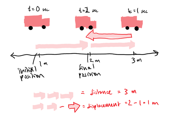
Position(x): location of an object at a specific time relative to the chosen origin Distance(d): how much ground has an object covered while it was moving
Displacement (Δx): net (overall) change in position
|
Position Time Graphs
Position Time Graphs - Interpretation
In a position-time graph, the vertical axis (independent variable) is the time and the horizontal axis (dependent variable) is the position of the object in motion. By plotting data points of the position of the object across a period of time, one can generate this type of graph.
Interpretation
Interpretation
- Initial Position (xi) = Y-value of graph at initial time
- Final Position (xf) = Y-value of graph at final time
- Displacement (Change in Position) (Δx) = final position - initial position
- Distance (d)= total of all changes in the y-value
- Change in Time (Δt) = final time - initial time
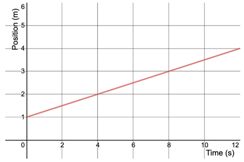
Example:
The position-time graph above depicts a person walking in a straight line. Interpretation
|
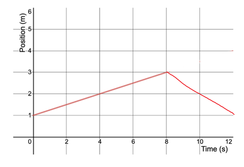
Example:
The position-time graph above depicts a person walking in a straight line, but they change direction at 8 seconds and walk faster. Interpretation
|
Position Time Graphs - Velocity & Speed
|
The position-time graph on the left depicts a person walking in a straight line from a position at 5 m to 0 m. Their displacement is -5 m and their change in time is 5 s, so their velocity is -5 m/s. However, the speed is 5 m/s because it does not include direction. |
Position Time Graphs - Determining Acceleration & Starting Velocity
- Acceleration (a)= whether the graph is a straight line or curved
- straight line = linear model = no acceleration (a = 0)
- curved = potentially quadratic, cubic, etc. model = acceleration
- concave up = positive acceleration (a > 0)
- concave down = negative acceleration (a < 0)
- Starting Velocity (vi) = steepness of slope at the beginning of the graph
- very steep = very high starting velocity
- flat = starting velocity is 0 m/s
|
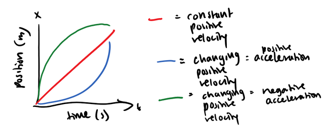
Example:
The graph in red indicates an object that has a constant positive velocity with no acceleration as its slope does not change. Its starting velocity is 0 m/s. Example:
The graph in blue indicates an object that has changing positive velocity with positive acceleration as its slope is becoming more and more steep and it is concave up. Its starting velocity is 0 m/s. Example:
The graph in green indicates an object that has changing positive velocity with negative acceleration as its slope is becoming less and less steep and it is concave down. Its starting velocity is very high as it is very steep. |
Velocity Time Graphs
Velocity Time Graphs - Interpretation
In a velocity-time graph, the vertical axis (independent variable) is the time and the horizontal axis (dependent variable) is the velocity of the object in motion. By plotting data points of the velocity of the object across a period of time, one can generate this type of graph.
Interpretation
Interpretation
- Initial Velocity (vi)= Y-value of graph at initial time
- Final Velocity (vf) = Y-value of graph at final time
- Speed (v)= absolute value of Y-value
- Average Velocity = (initial velocity + final velocity) / 2
- Direction (d) = positive (above the x-axis) or negative (below the x-axis)
- Acceleration (a)= change in velocity/ change in time
- Change in Time (Δt) = final time - initial time
|
|
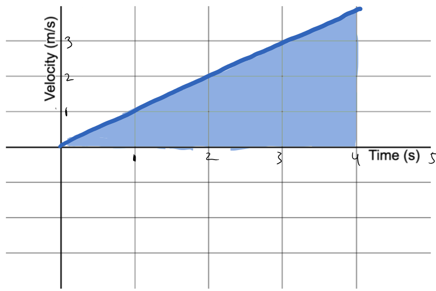
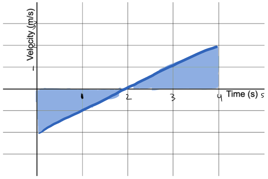
Velocity Time Graphs - Position, Distance, and Displacement
- Position (x)
- We don't know initial position or final position just by looking at the graph, but we know how much the position has change relative to each other by looking at the displacement
- Distance (d) = total area under curve of parts above or below the x-axis
- Displacement (Δx) = area under curve above x-axis - area under curve below x-axis
Example:
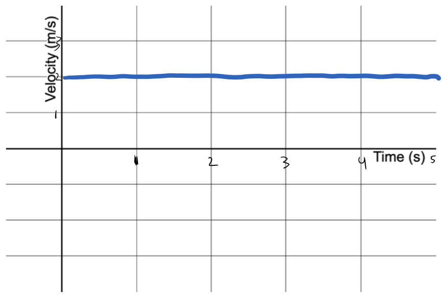
The graph above depicts the velocity of a person that is speeding up their walking. Interpretation
|
Example:
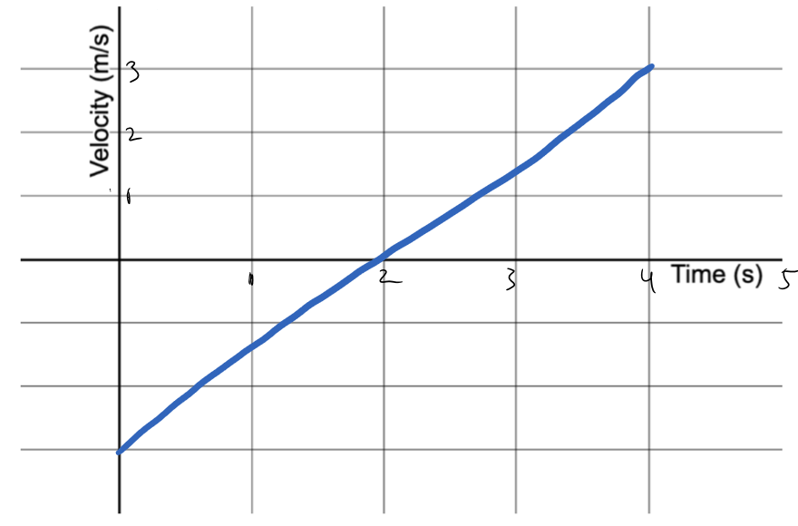
The graph above depicts the velocity of a person that is moving backward and slowing down from a race. They slow down to a velocity of 0 m, but realize that they are going in the wrong direction, so they turn around and move forward while speeding up. Interpretation
|
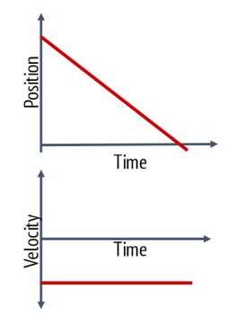
Connecting Representations of Motions
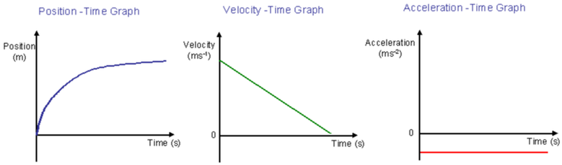
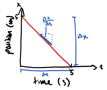
We can use the position time graph to determine the velocity by finding its slope, then use the velocity time graph to determine the acceleration by finding that slope. Conversely, we can find the area between the x-axis and the line for acceleration to create a velocity time graph, then find the area between the x-axis and the velocity graph to create a position time graph. However, without additional information, exact initial position cannot be identified from a velocity time graph or acceleration time graph.
|
|
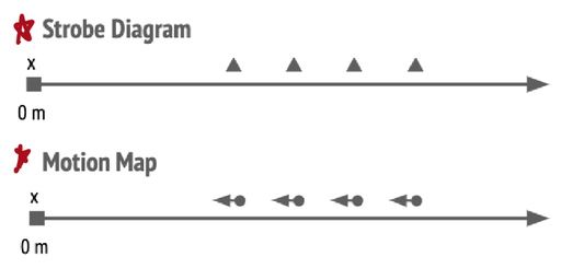
Strobe diagrams tell us the position of an object in motion over a period of time. With the arrows on the motion map, we know which direction the object is traveling in. Thus, we can create a position time graph with that information, then subsequent velocity time graphs and acceleration time graphs as described above.
Solving Kinematics Equations
Using constant velocity and uniform acceleration models.
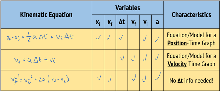
The three kinematic equations above all include different variations of the six variables
- initial position (xi)
- final position (xf)
- change in time (Δt)
- initial velocity (vi)
- final velocity (vf)
- acceleration (a)
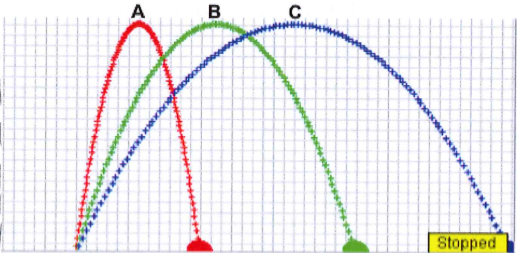
Projectile Motion
Projectile = an object in the air that is not acting upon the air
- has both horizontal and vertical motion
- Horizontal motion = how far the projectile travels
- Vertical motion = how long the projectile is in the air
- Speed = change in horizontal motion and vertical motion
|
The graph on the right shows three different projectiles each with the same vertical distance traveled, which indicates that they all spent the same amount of time in the air, but different horizontal distance, which indicates that their horizontal speeds were different.
Projectile C has the greatest speed because it traveled the furthest in the same amount of time as the other projectiles. |
